- Published on
Solving Travelling Salesman Problem With Variable Neighborhood Search
- Authors

- Name
- Ahmed Mrabet
- @Braatet
Introduction
The Travelling Salesman Problem (TSP) revolves around a simple query: Given a list of cities and the distances between each pair of cities, what is the shortest possible route that visits each city exactly once and returns to the origin city? Despite its seemingly straightforward premise, TSP is notoriously difficult to solve. This article explores how Variable Neighborhood Search (VNS) can effectively find approximate solutions to this complex problem.
- The Complexity of TSP: A Deep Dive
- Why Approximate Methods?
- Variable Neighborhood Search (VNS): A Comprehensive Breakdown
- Turning Theory into Python Code
- Evaluating VNS with Real-world TSP Problems
- Concluding Analysis
- Support
- License
The Complexity of TSP: A Deep Dive
Imagine you're a traveling salesman starting with a map and a simple task: to find the shortest path that covers all cities and returns home. At first glance, it may appear trivial, but the devil lies in the details.
The brute-force approach to solving TSP would be to evaluate every possible route and select the shortest. For a small number of cities, this might work, but as we add more cities to our list, the number of routes grows factorially. In computational terms:
- With 3 cities (ignoring the starting point for simplicity), there are 3! (3 factorial) possible routes, which is 3 x 2 x 1 = 6.
- With 4 cities, it's 4! or 4 x 3 x 2 x 1 = 24.
- With 5 cities, 5! equals 120 possible routes.
The growth rate is alarming. By the time you're dealing with:
- 10 cities, you have 3,628,800 possible routes.
- 15 cities, that number jumps to 1,307,674,368,000.
- 20 cities, the staggering 2,432,902,008,176,640,000 possible routes are to be examined!
This factorial growth means that even with supercomputers, solving a relatively modest TSP instance exactly can be infeasible.
Why Approximate Methods?
Given this complexity, it's clear that for larger instances of TSP, exact methods are impractical. This is where heuristic and metaheuristic methods come into play. These methods do not guarantee an optimal solution but can often find a very good (near-optimal) solution in a fraction of the time exact methods would take.
Metaheuristics like evolutionary algorithms are particularly interesting. These algorithms, inspired by natural processes, combine exploration (searching new areas of the solution space) and exploitation (refining promising areas). By maintaining a balance between these two aspects, they avoid getting trapped in local optima while not spreading their efforts too thinly across the vast solution space.
Variable Neighborhood Search (VNS): A Comprehensive Breakdown
Overview
The Variable Neighborhood Search (VNS) is a metaheuristic method designed to find approximate solutions to combinatorial optimization problems. Instead of remaining confined to a singular neighborhood during the search process, VNS ventures out, systematically exploring various neighborhood structures. This dynamic methodology is key to VNS's ability to avoid local optima and strive towards global optima.
Components of VNS
Multiple Neighborhood Structures: A key characteristic of VNS is its use of different neighborhood structures. These structures define how the search space around a solution can be modified. For example, in the context of TSP, one neighborhood structure might involve swapping two cities in the route, while another could reverse a segment of the route. If N₁, N₂, …, Nₖ are the k different neighborhood structures, then for a given solution s, Nₖ(s) denotes the k-th neighborhood of s.
Shaking Phase: The purpose of this phase is to push the search process out of local optima. It involves randomly selecting a solution from the k-th neighborhood of the current solution.
Local Search Phase: After the shaking phase, the solution might not be optimal within its neighborhood. So, a local search is applied to refine it. The local search explores the neighborhood of the perturbed solution and seeks a local optimum.
Update Phase: If the new solution found (after local search) is better than the current solution, the current solution is replaced with the new solution. This phase is crucial for maintaining the progression towards optimal or near-optimal solutions.
Working Principle
The VNS algorithm begins with an initial solution s and then repeats the following steps:
- Shaking: Select a neighborhood structure at random from the set N₁, N₂, …, Nₖ. Apply the shaking process to get a new solution s'.
- Local Search: From s', perform a local search to obtain s''.
- Update: If s'' is better than s, then update s = s''.
The algorithm terminates when a stopping criterion is met, such as a maximum number of iterations without improvement or a time limit.
Turning Theory into Python Code
Now that we've understood the mechanics of the Variable Neighborhood Search, let's translate that understanding into a Python program. Moreover, to gauge the efficacy of the algorithm, we'll use a benchmark dataset and compare our results. You can find the code in this repository:
Setting the Stage
Before diving into the algorithm, we have some utility functions and imports to aid in the process:
import random
import time
Fundamental Concepts & Corresponding Functions
Tour Distance
Given a tour (sequence of cities) and a distance matrix that denotes the distance between any two cities, this function calculates the total distance of that specific tour.
def tour_distance(tour, dist_matrix):
    return sum(dist_matrix[tour[i-1]][tour[i]] for i in range(len(tour)))
2-Opt Heuristic
The 2-opt heuristic is a simple yet effective local search method to refine a given route. It works by selecting two edges in the tour, reversing the cities between them, and then re-connecting the tour. This can lead to a shorter total distance.
def two_opt(tour, i, j):
    new_tour = tour[:i] + tour[i:j+1][::-1] + tour[j+1:]
    return new_tour
Local Search
At its heart, local search seeks to refine a given solution by looking at its neighborhood. Depending on the operation employed (like 2-opt), it iteratively tweaks the current solution in hopes of finding an improved one.
def local_search(tour, dist_matrix, operator):
    better_solution_found = True
    while better_solution_found:
        better_solution_found = False
        for i in range(1, len(tour) - 1):
            for j in range(i+1, len(tour)):
                if j-i == 1: continue
                new_tour = operator(tour, i, j)
                if tour_distance(new_tour, dist_matrix) < tour_distance(tour, dist_matrix):
                    tour = new_tour
                    better_solution_found = True
    return tour
Shaking
The shaking step introduces randomness into the algorithm. It essentially creates a new starting point by altering the existing solution. The idea is to escape local optima and explore new regions of the solution space.
def shaking(tour, k):
    new_tour = tour[:]
    for _ in range(k):
        i, j = sorted(random.sample(range(1, len(tour)-1), 2))
        new_tour = two_opt(new_tour, i, j)
    return new_tour
Variable Neighborhood Search (VNS)
VNS employs the principles of shaking and local search in tandem. After perturbing the current solution with shaking, VNS then applies local search to find a better solution in the new region. This dual approach ensures extensive exploration and intensive exploitation.
def vns(tour, dist_matrix, k_max=100, operator=two_opt):
    k = 1
    total_exploration_time = 0
    total_exploitation_time = 0
    while k <= k_max:
        time_start = time.time()
        k_tour = shaking(tour, k)
        time_end = time.time()
        total_exploration_time += time_end - time_start

        time_start = time.time()
        new_tour = local_search(k_tour, dist_matrix, operator)
        time_end = time.time()
        total_exploitation_time += time_end - time_start

        if tour_distance(new_tour, dist_matrix) < tour_distance(tour, dist_matrix):
            tour = new_tour
            k = 1
        else:
            k += 1
    return tour, total_exploration_time, total_exploitation_time
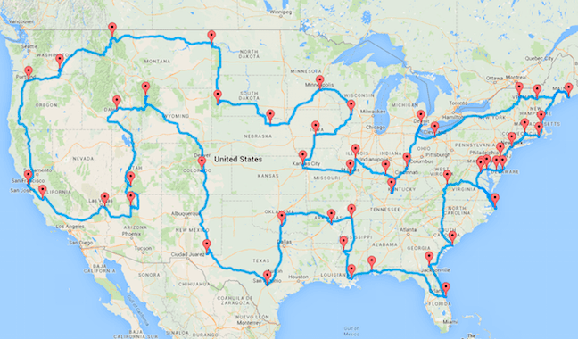
Evaluating VNS with Real-world TSP Problems
To truly validate the efficacy of the Variable Neighborhood Search (VNS) algorithm, it's essential to test it on real-world datasets. Thus, we've undertaken an evaluation on a diverse set of 10 Traveling Salesman Problem (TSP) instances. These problems vary in complexity, with the number of cities ranging from a mere 5 to a more challenging 280.
The primary metrics we're interested in are:
- The total distance achieved by the VNS algorithm.
- The deviation from the known optimal distance.
- The execution time, further broken down into exploration and exploitation times.
We also employ a visualization in the form of a chart graph to aid in the comprehension of the results.
Performance Overview
The VNS algorithm achieved an average score of 97.41%, when evaluated against the optimal solutions across the 10 datasets. This means that, on average, our VNS-derived solutions are 97.41% as good as the optimal ones.
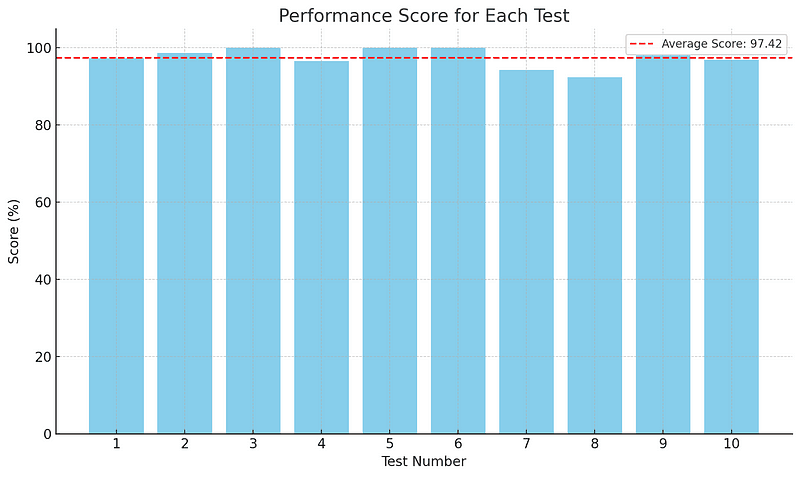
From this visualization, we can observe:
- The VNS algorithm has achieved 100% score (i.e., matched the optimal solution) in multiple tests.
- The performance is relatively consistent across tests, with most scores hovering near or above the average score.
Next, we'll visualize the total distance determined by the VNS algorithm vs. the optimal distance for each test.
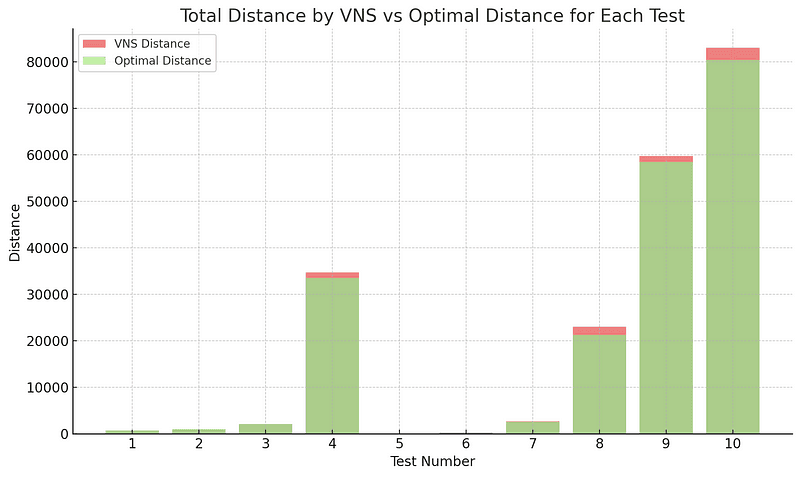
It's evident from the chart that in most tests, the VNS algorithm performs closely to the optimal solution, with only minor deviations in some cases.
Let's try visualizing the performance score as a function of the number of cities.
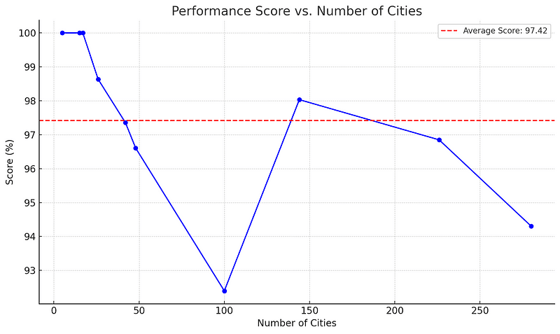
From this visualization, we can observe:
- Even as the number of cities increases, the VNS algorithm tends to deliver high scores. This is indicative of its ability to handle increased complexity.
- There is some variability in scores, especially in mid-sized problems. However, the scores remain relatively high across all sizes.
Next, let's visualize how the solution quality (total distance determined by VNS vs. optimal distance) varies with the number of cities.
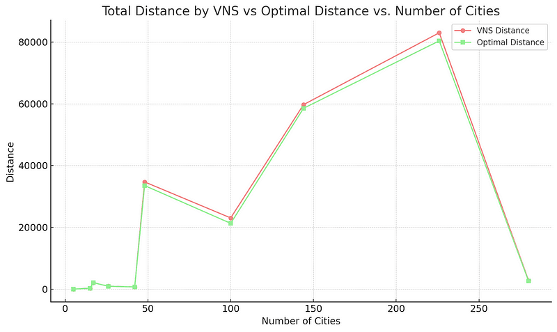
In several cases, especially for smaller problem sizes, the VNS algorithm's solution (in light red) closely converges with the optimal solution (in light green). This indicates that the VNS algorithm can find optimal or near-optimal solutions for these instances. As the number of cities (problem complexity) increases, there's a noticeable gap between the VNS distance and the optimal distance. However, this gap is relatively small, indicating that even for larger problems, the VNS algorithm is providing solutions close to the optimal.
Lastly, let's analyze how the execution time of the VNS algorithm scales with the number of cities.
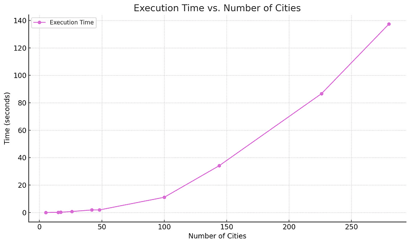
The execution time grows non-linearly with the number of cities. This behavior mirrors the combinatorial nature of the TSP. As the number of cities increases, there's a noticeable rise in execution time. This highlights the increased computational demand posed by larger TSP instances.
Concluding Analysis
Performance vs. Complexity: The VNS algorithm maintains high performance scores even as the number of cities (problem complexity) increases. While there is some variability in scores, especially for mid-sized problems, the VNS algorithm consistently delivers solutions close to the optimal.
Solution Quality: The VNS algorithm can find optimal or near-optimal solutions for many instances. However, as the problem size grows, there's a minor yet noticeable gap between the VNS solution and the optimal, indicating room for further improvement in larger problems.
Computational Time: The execution time grows non-linearly with the number of cities, highlighting the increased computational effort required for larger TSP instances.
Overall, the VNS algorithm showcases robust performance across various TSP sizes, making it a strong contender for solving TSP instances. However, for very large problems, considering the execution time and the minor deviation from the optimal solution, hybrid strategies or further algorithmic optimizations may be beneficial.
Support
Using the VNS algorithm for TSP? Support this effort by giving a star on GitHub, sharing your own implementations, or reaching out with feedback.